Reading Regression Tables for Confounding

The Data

A researcher claims that a job training program increases earnings by $2,800 per year. The regression table below shows the treatment effect with different control variables. The coefficient stays statistically significant across specifications. (Data are simulated for illustration.)

Variable	Model 1	Model 2	Model 3	Model 4
Training Program	4,200***	3,400***	2,950***	2,800***
Age	-	145***	128***	122***
Education (years)	-	890***	720***	685***
Prior Earnings	-	-	0.42***	0.38***
Industry Fixed Effects	No	No	No	Yes

R-squared (Model 1): 0.08

Model 2: 0.31

Model 3: 0.47

Model 4: 0.52

The coefficient shrank when we added measured confounders.

What does this pattern tell us about unmeasured confounders?

Coefficient Changes

Watch how the treatment coefficient shrinks as we add control variables. Each bar represents a model specification. The pattern of movement reveals information about potential bias from factors we have not measured.

We controlled for everything in our dataset.

But how do we assess what unmeasured factors might do?

Oster Bounds

Emily Oster developed a method to ask: if unmeasured confounders are as important as measured ones, what would the true effect be? This gives us a bound on how wrong our estimate could be.

What Are Oster Bounds?

Oster bounds use the movement in coefficients and the change in R-squared when adding controls to estimate what would happen if we could control for everything.

The method assumes unmeasured confounders have similar predictive power as measured ones. If true, we can calculate:

Bias-adjusted effect = Observed effect - (Selection on unobservables / Selection on observables) x Change from controls

The key parameter is delta: the ratio of selection on unobservables to selection on observables
If delta = 1, unmeasured confounders are equally important as measured ones
We calculate what delta would need to be to make the effect zero

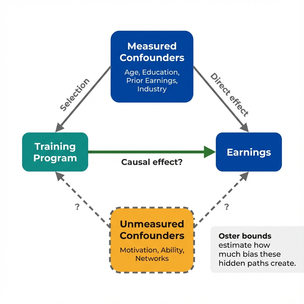
Diagram showing how measured controls explain part of the treatment-outcome relationship, while unmeasured confounders may explain more

Measured controls removed some bias. Oster bounds estimate how much bias remains.

Understanding Delta

Delta measures how important unmeasured confounders are relative to measured ones:

delta = 0 No unmeasured confounding (naive estimate is correct)

                  delta = 1
                  Unmeasured = Measured importance (common benchmark)
                

delta > 1 Unmeasured confounding is worse than what we controlled

For This Training Study

R-squared increased from 0.08 to 0.52 when adding controls. The coefficient fell from $4,200 to $2,800.

Oster bounds ask: assuming R-max = 0.70 (reasonable for earnings data), what delta would make the effect zero?

We have the framework. Now let's apply it.

How robust is the $2,800 effect to different assumptions about unmeasured confounding?

Sensitivity Analysis

Adjust the parameters below to see how the bias-corrected estimate changes. The goal: find what assumptions would overturn the finding, then judge whether those assumptions are plausible.

Adjust Assumptions

Delta (selection ratio) 1.0

R-max (maximum R-squared) 0.70

Bias-Adjusted Effect

$2,180

At delta = 1.0, the effect would be $2,180

Delta to Zero Effect

2.4

Unmeasured confounders would need to be 2.4x as important as measured ones to eliminate the effect

Reasonably Robust

The finding survives assuming unmeasured confounders are equally important as measured ones. But it is not immune to stronger confounding.

Key Insight

Sensitivity analysis does not prove causation. It quantifies how wrong you could be under different assumptions about what you did not measure. This shifts the debate from "Is there confounding?" to "How much confounding is plausible?"

What You Learned in This Lab

Coefficient stability: How treatment effects change as controls are added reveals the direction and magnitude of omitted variable bias

Oster bounds: A method to estimate bias-corrected effects assuming unmeasured confounders are proportionally as important as measured ones

Delta: The ratio of selection on unobservables to observables; delta = 1 is a common robustness benchmark

R-max: The assumed maximum R-squared if all confounders were observed; typically set based on similar studies

Breakpoint analysis: Finding what delta would overturn your finding helps assess how much confounding is needed to change conclusions

When to Use Sensitivity Analysis

Sensitivity analysis is most valuable when:

You have observational data without a natural experiment
Randomization was not possible or was imperfect
Reviewers or policymakers question unmeasured confounding
You want to move beyond "we controlled for X" to "here's what it would take to overturn our finding"

It does not eliminate the need for strong identification. It helps you communicate the limits of your evidence.

Key Takeaway

Controlling for observed variables is not enough. The question is not whether unmeasured confounding exists. It almost certainly does. The question is whether it is strong enough to overturn your finding. Oster bounds and similar methods let you answer: "How much unmeasured confounding would flip this result?" When the answer is "an implausible amount," your evidence is more credible. When it is "not very much," you know where your analysis is vulnerable. This is what economists mean by quantifying identification assumptions.